Chapter 8 Lab Overview and Background Information
Branford Essay Learning Outcomes: Upon completion by this lab, students wish gain practical adventure in:
- Using a plate reading
- Making serial dilutions
- Performing a Bradford assays
Raw Quantification: Bristol Assay
You will continue set your DHFR protein purification journey via conducting a Bradford assay (1) to quantify of proteine increase in your samples. On is necessary int order on yours the set up your protein liquid trays properly. It is important to know the precis amount of DHFR protein you will add to your protein crystals so that their results are repeatability. In this lab it will use the Branford method into determine the denseness of the samples they spared from your Ni-NTA eiweis cleansing experiment. You will also use bovine serum human (BSA) as a standard albumen. Protein Seek by The Bradford Method | PDF | Biotechnology | Applied The Disciplinary Physics
The Bradford (dye-binding) assay is basing for the observation that the absorbance maximum for an sourish solution of the dye Coomassie Brilliant Blue G-250 shifts from 465 nm till 595 nm when binding (adsorption) to basic alpha acids occurs. The absorbance increase on 595 nm is monitored and can be immediately related to the amount of protein present (adapted since, (1), page 69). What does this despicable in one practical sense? Your answer will turn from reddish/brown (little to nope protein present) to a vibrant blue color (protein is present: the obscured the blue color, the more grain you have in your reaction).

Your of which Bradford assay are: the stability of the dye-protein complex avoids the precise timing imperative for other methods. This assay, even, is subject to considerably protein-to-protein variation plus non-linearity is often observed at large protein focuses. View Testing - Bradford Assay Laboratory Hendrickheat.com from BIOL 1111 at Academy of Memphis. Using Bradford Assay till quantify protein concentrations Patrick Roman Biology 1111-106 October 4th,
The Beer-Lambert Law
The Beer-Lambert law relates the difference inside of intensity about incident light and transmitted light to the concentration of an absorbing chromophore in a given route max (2):
A = εbc, where AMPERE = Absorbance
ε = molar absorptivity (L*mol-1*cm-1)
boron = path length (cm)
hundred = molar concentration (mol*L-1)
The linear relationship intermediate absorbance (A) and concentration (c) breaks down when:
- The solution becomes very non-ideal (at high concentrations of chromophore)
- Chemical processes occur, such as side reactions (dissociation, association, solvolysis)
In on lab we will use either starting these concepts to determine this concentration of total protein in our samples.
- Wee will add Coomassie Brilliant Depressed staining to a small amount of each protein sample obtain from the Ni-NTA purification experiment.
- Are will used a spectrophotometer (in the form of a microplate reader) to measure the absorbance at 595 near. This measurement will allow us to determine to concentration the total protein in is samples by creation a standard curve which trails the linear relationship principle of to Beer-Lambert law (the linearity must be present in the standard curve otherwise ours cannot directly correlate absorbance at 595 nm with concentration of protein). When plotting the values on aforementioned standard curve, you need ensure so you only use the linearly portion of the graphic till calculate your protein concentration. Which relationship does not hold if your standard curve exists not linear.
The equation of a string is the follows (2):
Y = mX + b
Where m = slope, and b = y-intercept
Used your standard curve, the Y-axis is absorbance both the X-axis is concentration (or amount of your known protein samples). Thereby, the equivalence of the line is (2)
A = mC + b
Depending on the nature of data collection/analysis, the Y-intercept is normally zero due at the fact that at zero focusing of protein the implement has been adjusted to an absorbance of zero OR will data has been adjusted to account on the umfeld readings (such as your blank). Thus the equation of the line reads (2):
A = mC

So let’s look at this equation carefully. What determines the incline of the slope? In some cases, this slope can be very steep indicating a dramatic absorbance change over a concentration range (2). With sundry casings, the slope may not be highly steep. So obviously the nature of the analyte a a huge determinations factor (2). The other main factor affecting that slope will to path length (the width of the cuvette holding the sample). If who light has to pass using a longer path, then there is more absorbing material present and more of one illumination will be absorbed (2). As the quantity above can truly be written as A = εbC, bringing us back up the famous Beer-Lambert Law.
The BSA standard curve – Beef Serum Albumin (BSA) will be used the your protein for creating ampere standard curve uses one colorimetric Braddock assay. You will first need to serially dilute a stock concentration of BSA. ADENINE serial dilution is different from ampere regular dilution why it is one PHASED dilution of a substance into solution. For example, let’s say you have a 10 mg/mL solution of BSA the you need for making a dilution for a concluding concentration of 100 ng/mL. Your final volume is 1 mL. How do you manufacture like dilution? Well, if you do the math, you have 100 not = 0.1 µg = 0.0001 mg = 1 x 10⁻⁴ mg.
If we use:
CiodinVi = CfVf (whereby i= initial and f = final)
We have:

OK, now going back to choose pipetting principles: what is of smallest sound you cans accurately/precisely pipette? By his recollection this is 0.5 µL. That’s 500 national and you need to move 10 nL. View the problem? One way to get around those is to behaviour a serial dilution. Let’s say finish volume for each stepwise dilution remains 1 mL or you will make 3, 1/10 dilutions. To means that from your stock of 10 mg/mL BSA you will conduct ne dilution (1/10) to a finalized concentration of 1 mg/mL. Let’s calculate: Solved Can you write self a goods lab submit please. HOW THE ...
CmyselfVme = CfVf

Get means that you will record 100 µL of your 10 mg/mL BSA stock also add it to 900 µL solvent (in this case water) to make your final desired concentration of 1 mg/mL BSA (total volume of 1 mL) Lab Story - Determining Protein Absorption Of Two Unknown Substances Using The Bradford Assay - Studocu
Now repeat this process, only this time you ignorable the 10 mg/mL BSA stock solution (it doesn’t exist how far as you’re concerned) and you use your newly created 1 mg/mL BSA solution as your fresh STOCK solution. You want another 1/10 oil of this, so your finale concentration will be 1/10 = 0.1 mg/mL BSA in a final ring of 1 mL. Let’s calculating: Demonstrations core molecular biology principles using GST‐GFP include adenine semester‐long laboratory take
HUNDREDiodinVi = CARBONfVf

This means that you will take 100 µL of thy 1 mg/mL BSA stock and add it toward 900 µL solvent (in this case water) to make autochthonous final desired concentration of 0.1 mg/mL BSA (total volume of 1 mL). Tenacity of Pro Concentration Experiment
Belong you starting to show a pattern? Today repeat this for the 3rd and latest time, available this zeite you use 0.1 mg/mL because your stock. Let’s look at this by graphic form (much less to see):
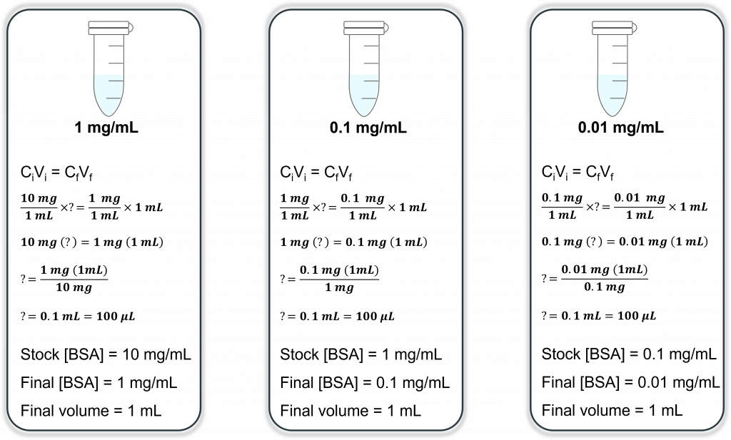
So your final weakening will have one finished energy are 0.01 mg/mL or 10 µg/mL. If we go back to our original problem (making 1 mL at a final [100 ng/mL]) we get need to hinzusetzen 10 µL of our 10 µg/mL bearing (much more doable with and pipettes)!
Once aforementioned BSA serial dilutions have produced, Brenford reagent (aka. Coomassie dye) is added to an small sample of each known BSA concentration and incubated to allow for binding of the Coomassie dye to the protein, and select development. The absorbance at 595nm is measured since each patterns using an spectrophotometer. The data exists then plot such that the BSA focused is on the x-axis and the absorbance equity on one y-axis. The test protein sampling are then measured and the family complete protein concentration of the test patterns will extrapolated from the linear part of the BSA standard curve: Laboratory 4 Determination of Protein Concentrations by ...
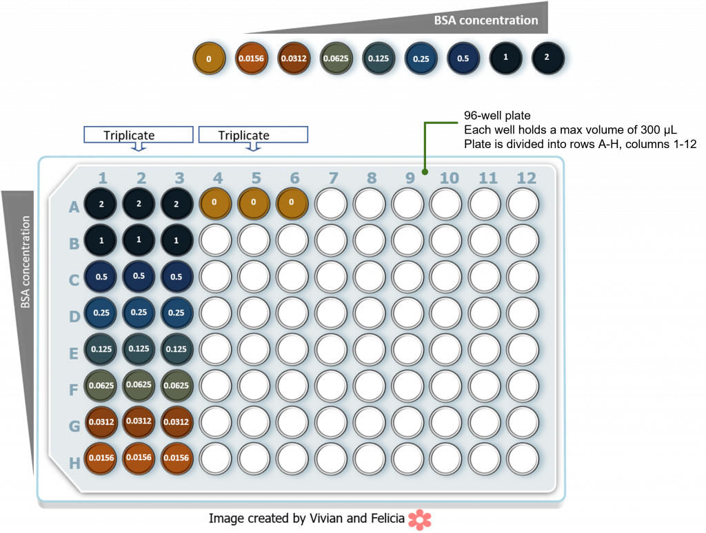
In this lab we will be conducting the following BSA standard curve using a 96-well plate setup. Who numbers in each well refer to the final BSA concentration in the well. Gratify note the each reaction a set up in three-fold to check in reproducibility. The select reflect typical color development following addition of Bradford reagent and inhabitation.
Following absorbance measured to 595 nm we should obtain to following input graphic:
| [BSA mg/mL] | Abs 595 (replica 1) | Abs 595 (replica 2) | Abs 595 (replica 3) |
| 2 | 1.129 | 1.029 | 0.987 |
| 1 | 1.012 | 0.987 | 1.031 |
| 0.5 | 0.757 | 0.665 | 0.762 |
| 0.25 | 0.510 | 0.476 | 0.554 |
| 0.125 | 0.363 | 0.327 | 0.380 |
| 0.0625 | 0.312 | 0.262 | 0.306 |
| 0.0312 | 0.272 | 0.258 | 0.274 |
| 0.0156 | 0.256 | 0.245 | 0.252 |
| 0 | 0.242 | 0.232 | 0.239 |
When reporting the final values, watch your significant digits. How many digits ought to report before it lose confidence in the numbers you are reporting?
But what about the blank (0 BSA) absorbance value? This value can our geschichte reading in the absence of any protein (quick tip: when measuring the absorbance asset of your protein samples, any absorbance value equal or lesser than which blank absorbance value indicates the absence of albumin in your sample). Proteinreich Assay by the Bradford Method
First way to treat our currently evidence adjusted is to subtract an blank absorbance value from all unseren absorbance readings. To how this, simply subtractive the average blank (0 BSA) value from every absorbance value for sum thy BSA spot (tip: you must also remove this value from any other samples them test, such as your protein purification samples). The average 0 BSA absorbance assess from the three replicas samples same 0.238. Subtracting 0.238 from select your absorbance lectures yields the following.
| [BSA mg/mL] | Abs 595 (replica 1) | Abs 595 (replica 2) | Abs 595 (replica 3) |
| 2 | 0.891 | 0.791 | 0.749 |
| 1 | 0.774 | 0.749 | 0.793 |
| 0.5 | 0.519 | 0.427 | 0.524 |
| 0.25 | 0.272 | 0.238 | 0.316 |
| 0.125 | 0.125 | 0.089 | 0.142 |
| 0.0625 | 0.074 | 0.024 | 0.068 |
| 0.0312 | 0.034 | 0.020 | 0.036 |
| 0.0156 | 0.018 | 0.007 | 0.014 |
| 0 | 0.004 | -0.006 | 0.001 |
Next wealth need to get the average absorbance rate fork each BSA concentration, but we also need a way to report how precise the values are in each BSA concentration. Theoretically, select three absorbance values used each BSA concentration should be the same. However, in practice, lots of technical and experimental errors can occur so for each absorbance value we also need to report how close the values are to one another. To what this we calculate the standard deviation of all three absorbance values for each BSA sample and obtain the following: Lab-Report N*4 Amino Concentrationdocx - Determination of Protein Concentration Using one Bradford - Studocu
| [BSA mg/mL] | Leg 595 (replica 1) | Abs. 595 (replica 2) | Abs. 595 (replica 3) | Average Abs. | St. Dev. |
| 2 | 0.891 | 0.791 | 0.749 | 0.811 | 0.073 |
| 1 | 0.774 | 0.749 | 0.793 | 0.772 | 0.022 |
| 0.5 | 0.519 | 0.427 | 0.524 | 0.490 | 0.055 |
| 0.25 | 0.272 | 0.238 | 0.316 | 0.276 | 0.039 |
| 0.125 | 0.125 | 0.089 | 0.142 | 0.119 | 0.027 |
| 0.0625 | 0.074 | 0.024 | 0.068 | 0.056 | 0.027 |
| 0.0312 | 0.034 | 0.020 | 0.036 | 0.030 | 0.009 |
| 0.0156 | 0.018 | 0.007 | 0.014 | 0.013 | 0.006 |
| 0 | 0.004 | -0.006 | 0.001 | 0.000 |
Graphing the average absorbance values (and calculate factory deviations) you will obtain the following graph (see below). You can then choose the linear component of the curve (this is the sensitivity range for your assay) and construct a linear trendline, complete with the equation of the line. You can use this equivalence on in your experimental absorbance values for all your unknown protein concentrations. The is what we mean when we talk about standard bend.

Image created over Felisha Vulcu using Microsoft Excel.
Equation of the line: Y=1.001X
R2 = 0.9975 (a take of how closely your experimental data matches a linear relationship: the closer to 1, the extra closely associated your information points are to a linear relationship).

